Chapter 3 R Programming language primer

The R programming language comprises 6 major types of R objects

• Vectors
• Matrix
• Data Frame
• Lists
• Array
• Factors

3.1 Vectors

The vector type is the fundamental data type in R. The elements of a vector must all have the same mode (data type) of the following type:

• Scalars are individual numbers, they actually are one-element vectors e.g. x <- 10
• Character strings are single-element vectors of mode ”character” e.g. y <- "hello"

x <- c(1, 2, 3, 4, 5, 6)
x
#> [1] 1 2 3 4 5 6
x <- 1:6
x
#> [1] 1 2 3 4 5 6
x[1]
#> [1] 1
text <- c("Hello",  "World")
text
#> [1] "Hello" "World"
names(x) <- paste("name", 1:6, sep="")
x
#> name1 name2 name3 name4 name5 name6 
#>     1     2     3     4     5     6

3.1.1 Vectors in action

z_scores <- seq(-3, 3, by = .1)
z_scores
#>  [1] -3.0 -2.9 -2.8 -2.7 -2.6 -2.5 -2.4 -2.3 -2.2 -2.1 -2.0 -1.9 -1.8 -1.7
#> [15] -1.6 -1.5 -1.4 -1.3 -1.2 -1.1 -1.0 -0.9 -0.8 -0.7 -0.6 -0.5 -0.4 -0.3
#> [29] -0.2 -0.1  0.0  0.1  0.2  0.3  0.4  0.5  0.6  0.7  0.8  0.9  1.0  1.1
#> [43]  1.2  1.3  1.4  1.5  1.6  1.7  1.8  1.9  2.0  2.1  2.2  2.3  2.4  2.5
#> [57]  2.6  2.7  2.8  2.9  3.0
norm.dist <- dnorm(z_scores)
norm.dist
#>  [1] 0.004431848 0.005952532 0.007915452 0.010420935 0.013582969 0.017528300
#>  [7] 0.022394530 0.028327038 0.035474593 0.043983596 0.053990967 0.065615815
#> [13] 0.078950158 0.094049077 0.110920835 0.129517596 0.149727466 0.171368592
#> [19] 0.194186055 0.217852177 0.241970725 0.266085250 0.289691553 0.312253933
#> [25] 0.333224603 0.352065327 0.368270140 0.381387815 0.391042694 0.396952547
#> [31] 0.398942280 0.396952547 0.391042694 0.381387815 0.368270140 0.352065327
#> [37] 0.333224603 0.312253933 0.289691553 0.266085250 0.241970725 0.217852177
#> [43] 0.194186055 0.171368592 0.149727466 0.129517596 0.110920835 0.094049077
#> [49] 0.078950158 0.065615815 0.053990967 0.043983596 0.035474593 0.028327038
#> [55] 0.022394530 0.017528300 0.013582969 0.010420935 0.007915452 0.005952532
#> [61] 0.004431848
mean(norm.dist)
#> [1] 0.1635609
median(norm.dist)
#> [1] 0.1295176
sd(norm.dist)
#> [1] 0.140773

3.2 Matrix

A matrix is a rectangular array of numbers (technically a vector with a number of rows and a number of columns)

m <- matrix(x, nrow = 2)
m
#>      [,1] [,2] [,3]
#> [1,]    1    3    5
#> [2,]    2    4    6

m <- matrix(x, nrow = 2, byrow = TRUE)
m
#>      [,1] [,2] [,3]
#> [1,]    1    2    3
#> [2,]    4    5    6

3.2.1 Matrices in action

normMat <- matrix(rnorm(10),nrow=5,ncol=20)
normMat[1:5,1:5]
#>            [,1]       [,2]       [,3]       [,4]       [,5]
#> [1,]  0.4608433 -1.2710462  0.4608433 -1.2710462  0.4608433
#> [2,] -0.6669574  0.9299691 -0.6669574  0.9299691 -0.6669574
#> [3,]  0.5542039 -0.7793734  0.5542039 -0.7793734  0.5542039
#> [4,] -0.4471556  1.3831410 -0.4471556  1.3831410 -0.4471556
#> [5,] -0.8371289 -0.5374330 -0.8371289 -0.5374330 -0.8371289
rownames(normMat) <- paste("Gene", 1:5, sep="_")
normMat[1:5,1:5]
#>              [,1]       [,2]       [,3]       [,4]       [,5]
#> Gene_1  0.4608433 -1.2710462  0.4608433 -1.2710462  0.4608433
#> Gene_2 -0.6669574  0.9299691 -0.6669574  0.9299691 -0.6669574
#> Gene_3  0.5542039 -0.7793734  0.5542039 -0.7793734  0.5542039
#> Gene_4 -0.4471556  1.3831410 -0.4471556  1.3831410 -0.4471556
#> Gene_5 -0.8371289 -0.5374330 -0.8371289 -0.5374330 -0.8371289
#Calculate mean for each matrix row
apply(normMat, MARGIN=1, mean)
#>     Gene_1     Gene_2     Gene_3     Gene_4     Gene_5 
#> -0.4051014  0.1315059 -0.1125847  0.4679927 -0.6872809
#Calculate mean for each matrix column
apply(normMat, MARGIN=2, mean)
#>  [1] -0.18723893 -0.05494848 -0.18723893 -0.05494848 -0.18723893 -0.05494848
#>  [7] -0.18723893 -0.05494848 -0.18723893 -0.05494848 -0.18723893 -0.05494848
#> [13] -0.18723893 -0.05494848 -0.18723893 -0.05494848 -0.18723893 -0.05494848
#> [19] -0.18723893 -0.05494848

3.3 Data Frame

A data frame is a data set that contains data of different modes (i.e. different types). A data frame is a list with each component of a list being a vector corresponding to a column in the data.

df <- data.frame(cancerType = c("PDAC", "PDAC", "PDAC"),  
  KRAS_status = c("wt", "mut", "mut"), Subtype = c("Classical", "Classical", "Subtype"))
df
#>   cancerType KRAS_status   Subtype
#> 1       PDAC          wt Classical
#> 2       PDAC         mut Classical
#> 3       PDAC         mut   Subtype

3.3.1 Data Frames in action

#Extract cancerType
df[,1]
#> [1] PDAC PDAC PDAC
#> Levels: PDAC
#Extract cancerType
df$cancerType
#> [1] PDAC PDAC PDAC
#> Levels: PDAC
#Assigning new data
df$Sex  <- c("Male", "Female", "Male")
df
#>   cancerType KRAS_status   Subtype    Sex
#> 1       PDAC          wt Classical   Male
#> 2       PDAC         mut Classical Female
#> 3       PDAC         mut   Subtype   Male
#Excluding factors
df <- data.frame(cancerType = c("PDAC", "PDAC", "PDAC"),  
  KRAS_status = c("wt", "mut", "mut"), Subtype = c("Classical", "Classical", "Subtype"), stringsAsFactors = FALSE)
df$cancerType
#> [1] "PDAC" "PDAC" "PDAC"

3.4 Factors

Factors are used to represent categorical data. Factors can be ordered or unordered and are an important class for statistical analysis and for plotting.

subtype <- factor(c("Classical", "Basal", "Basal", "Classical"))
subtype
#> [1] Classical Basal     Basal     Classical
#> Levels: Basal Classical
levels(subtype)
#> [1] "Basal"     "Classical"
table(subtype)
#> subtype
#>     Basal Classical 
#>         2         2

3.4.1 Factors in action

colours <- c("red", "green")
colours[subtype]
#> [1] "green" "red"   "red"   "green"

3.5 List

Lists can contain items comprising different data types and are similar to a C struct in C++.

list1 <- list(1:20, "KRAS", list(1:6, 7:10))
list1
#> [[1]]
#>  [1]  1  2  3  4  5  6  7  8  9 10 11 12 13 14 15 16 17 18 19 20
#> 
#> [[2]]
#> [1] "KRAS"
#> 
#> [[3]]
#> [[3]][[1]]
#> [1] 1 2 3 4 5 6
#> 
#> [[3]][[2]]
#> [1]  7  8  9 10

3.5.1 Lists in action

list2 <- list(rnorm(10), rnorm(10), rnorm(10))
#Access first entry of list2
list2[1]
#> [[1]]
#>  [1]  0.2865250  1.6296273 -1.7738138 -0.4006902  0.0556799 -0.8535119
#>  [7] -2.2770253 -0.6963454  0.3484086  0.6402198
#Access vector of values in first entry of list2
list2[[1]]
#>  [1]  0.2865250  1.6296273 -1.7738138 -0.4006902  0.0556799 -0.8535119
#>  [7] -2.2770253 -0.6963454  0.3484086  0.6402198
#Finding mean for each vector series in list2 - returns a list of means
lapply(list2, mean)
#> [[1]]
#> [1] -0.3040926
#> 
#> [[2]]
#> [1] -0.4322401
#> 
#> [[3]]
#> [1] 0.4697256
#Finding mean for each vector series in list2 - returns a vector of means
sapply(list2, mean)
#> [1] -0.3040926 -0.4322401  0.4697256

3.6 Array

Arrays are matrices with more than 2 dimensions.

ar <- array(c(11:14, 21:24, 31:34), dim = c(2, 2, 3))
ar
#> , , 1
#> 
#>      [,1] [,2]
#> [1,]   11   13
#> [2,]   12   14
#> 
#> , , 2
#> 
#>      [,1] [,2]
#> [1,]   21   23
#> [2,]   22   24
#> 
#> , , 3
#> 
#>      [,1] [,2]
#> [1,]   31   33
#> [2,]   32   34

3.7 Creating functions

#Function to select the top n most variable genes
rnaSelectTopVarGenes <- function(normCounts, n=2000){
  mad <- apply(normCounts, 1, mad)
  ords <- names(sort(mad, decreasing=TRUE))
  select <- normCounts[ords[1:n],]
  select
}

top2varGenes <- rnaSelectTopVarGenes(normMat, n=2)
head(top2varGenes)
#>              [,1]      [,2]       [,3]      [,4]       [,5]      [,6]
#> Gene_4 -0.4471556  1.383141 -0.4471556  1.383141 -0.4471556  1.383141
#> Gene_1  0.4608433 -1.271046  0.4608433 -1.271046  0.4608433 -1.271046
#>              [,7]      [,8]       [,9]     [,10]      [,11]     [,12]
#> Gene_4 -0.4471556  1.383141 -0.4471556  1.383141 -0.4471556  1.383141
#> Gene_1  0.4608433 -1.271046  0.4608433 -1.271046  0.4608433 -1.271046
#>             [,13]     [,14]      [,15]     [,16]      [,17]     [,18]
#> Gene_4 -0.4471556  1.383141 -0.4471556  1.383141 -0.4471556  1.383141
#> Gene_1  0.4608433 -1.271046  0.4608433 -1.271046  0.4608433 -1.271046
#>             [,19]     [,20]
#> Gene_4 -0.4471556  1.383141
#> Gene_1  0.4608433 -1.271046

3.8 Loading Data

Loading data from a comma separated file can be easily achieved using the read.delim or read.csv functions. There are many alternatives!

moffitt <- read.delim("course/Moffitt_gene_signature.csv", 
                      sep=",", stringsAsFactors = FALSE)
head(moffitt)
#>     symbol     Group
#> 1    MUC13 Classical
#> 2    GPR35 Classical
#> 3    USH1C Classical
#> 4 BAIAP2L2 Classical
#> 5  GAL3ST1 Classical
#> 6     VIL1 Classical
class(moffitt)
#> [1] "data.frame"
moffitt$symbol
#>  [1] "MUC13"      "GPR35"      "USH1C"      "BAIAP2L2"   "GAL3ST1"   
#>  [6] "VIL1"       "DDC"        "LGALS4"     "TSPAN8"     "SLC5A1"    
#> [11] "SEMA4G"     "TNFRSF11A"  "HSD17B2"    "CKMT1A"     "DPCR1"     
#>  ...
#> [76] "REEP3"      "DCBLD2"     "NMB"        "IKZF2"      "GPR87"     
#> [81] "MUC16"      "IVL"        "SPRR1B"     "BCAR3"      "TTC9"      
#> [86] "PTGES"      "CST6"       "CATSPER1"

3.9 Saving Data

Saving data is also simple. You can write data to comma separated (csv) files using the write.table function.

The best way to store objects from R is within .RData files. .RData files are specific to R and can store as many objects as required.

#Write data to a tab separate file called Moffitt_gene_signature.tsv
write.table(moffitt, "course/Moffitt_gene_signature.tsv", 
            sep="\t", quote = FALSE, row.names = FALSE)
#Save moffitt to a RData file called moffittSig.RData
save(moffitt,x,y,z,file="course/moffittSig.RData")
#Load themoffitt data.frame into the current environment
load("course/moffittSig.RData")

3.10 Saving plots

How do we save complex plots like the one below?

df <- 6 - 1
f <- function(x) {
  dt(x, df)
}
plot(f, -4, 4, xlab = "x-axis", ylab = "T Density dt(x)")
ci <- c(qt(0.025, df), qt(0.975, df))
x <- seq(-4, ci[1], 0.01)
y <- seq(ci[2], 4, 0.01)
polygon(c(ci[1], x, ci[1]), c(0, 0, f(x)), col = "red")
polygon(c(ci[2], y, ci[2]), c(f(y), 0, 0), col = "red")
arrows(-3, 0.25, -3, 0.05)
text(-3, 0.3, "Rejection Region")
arrows(3, 0.25, 3, 0.05)
text(3, 0.3, "Rejection Region")
arrows(0, 0.15, 0, 0.05)
text(0, 0.2, "Acceptance Region")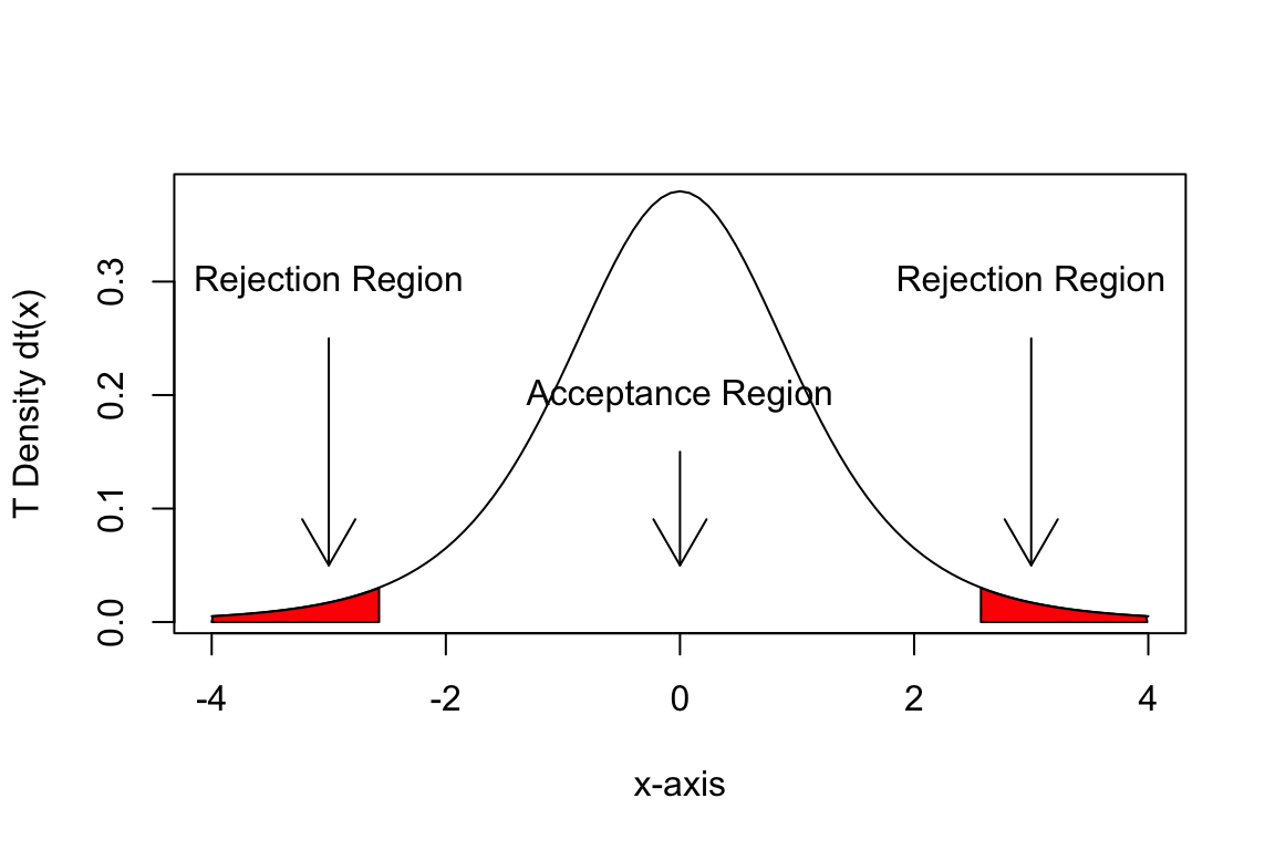

Figure 3.1: Acceptance and rejection regions in a t-test distribution.

It is easy to save the above plot using the pdf() and dev.off() functions as follows. All of the plotting commands contained between the pdf() & dev.off() functions will be sent to file. It is also possible to use the png() function if you would like to create png’s instead! Check out the grDevices package for other alternatives.

pdf("course/normalDist.pdf", height=6, width=4)
  df <- 6 - 1
  f <- function(x) {
    dt(x, df)
  }
  plot(f, -4, 4, xlab = "x-axis", ylab = "T Density dt(x)")
  ci <- c(qt(0.025, df), qt(0.975, df))
  x <- seq(-4, ci[1], 0.01)
  y <- seq(ci[2], 4, 0.01)
  polygon(c(ci[1], x, ci[1]), c(0, 0, f(x)), col = "red")
  polygon(c(ci[2], y, ci[2]), c(f(y), 0, 0), col = "red")
  arrows(-3, 0.25, -3, 0.05)
  text(-3, 0.3, "Rejection Region")
  arrows(3, 0.25, 3, 0.05)
  text(3, 0.3, "Rejection Region")
  qrrows(0, 0.15, 0, 0.05)
  text(0, 0.2, "Acceptance Region")
dev.off()