Chapter 6 RNAseq Analysis - DESeq2
In this Chapter, we will be analyzing RNAseq data previously published in Brunton et al. HNF4A and GATA6 Loss Reveals Therapeutically Actionable Subtypes in Pancreatic Cancer. Cell Reports 2020. The RNAseq experiment that we will re-analyse involves the Knock-Down (KD) of HNF4A using a specific siRNA in 2 different Patient Derived Cell Lines (PDCLs) Mayo5289 and TKCC22. Both Mayo5289 and TKCC22 are Classical lines which expresses HNF4A. We have 12 samples in total, representing:
- 3x Mayo5289 Scrambled Controls (Biological Replicates)
- 3x Mayo5289 siHNF4A (Biological Replicates)
- 3x TKCC22 Scrambled Controls (Biological Replicates)
- 3x TKCC22 siHNF4A (Biological Replicates)
RNAseq data has been mapped and a merged counts file is available for us to analyse. Let’s take a look at the sample sheet for the experiment.
sampleSheet <- read.delim("RNASeqData/SampleSheetBrunton.tsv", sep = "\t",
                          stringsAsFactors = FALSE)
sampleSheet
#>       id Treatment_group Batch
#> 1  HB.A1    TKCC-22_Cont     1
#> 2  HB.A3   TKCC-22_HNF4A     1
#> 3  HB.B1    TKCC-22_Cont     2
#>  ...<6 more rows>...
#> 10 HB.E3 Mayo_5289_HNF4A     2
#> 11 HB.F1  Mayo_5289_Cont     3
#> 12 HB.F3 Mayo_5289_HNF4A     3
The merged counts file is in the following format:
countsFile <- read.delim("RNASeqData/CountsFileBrunton.tsv",
                         stringsAsFactors = FALSE, sep = "\t",row.names = 1)
head(countsFile)
#>                 HB.A1 HB.A3 HB.B1 HB.B3 HB.C1 HB.C3 HB.D1 HB.D3 HB.E1 HB.E3
#> ENSG00000223972     0     0     0     0     0     0     1     0     0     0
#> ENSG00000227232   206   147   149   161   160   184   154   200   222   201
#> ENSG00000243485     0     0     0     0     0     0     0     0     0     0
#> ENSG00000237613     0     0     0     0     0     0     0     0     0     0
#> ENSG00000268020     0     0     0     0     0     0     0     0     0     0
#> ENSG00000240361     0     0     0     0     0     0     0     0     0     0
#>                 HB.F1 HB.F3
#> ENSG00000223972     0     0
#> ENSG00000227232   167   188
#> ENSG00000243485     0     0
#> ENSG00000237613     0     0
#> ENSG00000268020     0     0
#> ENSG00000240361     0     0
6.1 DESEq2 package
The DESeq2 package expects count data in the form of a matrix of integer values as input. The values in the matrix should be non-normalized counts or estimated counts of sequencing reads (for single-end RNA-seq) or fragments (for paired-end RNA-seq). The DESeq2 model internally corrects for library size, so transformed or normalized values such as counts scaled by library size should not be used as input.
The DESeq2 package stores the read counts and the results of any analysis in an object of class DESeqDataSet. The DESeqDataSet class extends the RangedSummarizedExperiment class of the SummarizedExperiment package, which we used previously in Section 4.2.
6.2 The DESeqDataSet
A DESeqDataSet object must have an associated design formula. The design formula expresses the variables which will be used in modeling. The formula should be a tilde (~) followed by the variables with plus signs between them (it will be coerced into an formula if it is not already).
6.3 Count matrix input
The function DESeqDataSetFromMatrix can be used to generate a RangedSummarizedExperiment object comprising our data. The Treatment_group sample sheet column is used for our design formula!
library(DESeq2)
## Produce a DESeq dataset
dds <- DESeqDataSetFromMatrix(countData = countsFile,
                              colData = sampleSheet,
                              design = ~ Treatment_group)
#> Warning in DESeqDataSet(se, design = design, ignoreRank): some variables in
#> design formula are characters, converting to factors
#>   Note: levels of factors in the design contain characters other than
#>   letters, numbers, '_' and '.'. It is recommended (but not required) to use
#>   only letters, numbers, and delimiters '_' or '.', as these are safe characters
#>   for column names in R. [This is a message, not an warning or error]
Let’s take a look at the colData for this object. The colData function will allow us to access the Treatment_group and experiment ids later on!
head(colData(dds))
#> DataFrame with 6 rows and 3 columns
#>                id Treatment_group     Batch
#>       <character>        <factor> <integer>
#> HB.A1       HB.A1    TKCC-22_Cont         1
#> HB.A3       HB.A3   TKCC-22_HNF4A         1
#> HB.B1       HB.B1    TKCC-22_Cont         2
#> HB.B3       HB.B3   TKCC-22_HNF4A         2
#> HB.C1       HB.C1    TKCC-22_Cont         3
#> HB.C3       HB.C3   TKCC-22_HNF4A         3
6.4 Pre-filtering
While it is not necessary to pre-filter low count genes before running the DESeq2 functions, there are two reasons which make pre-filtering useful:
- by removing rows in which there are very few reads, we reduce the memory size of the dds data object
- we increase the speed of the transformation and testing functions within DESeq2.
Here we perform a minimal pre-filtering to keep only rows that have at least 10 reads total. Note that more strict filtering to increase power is automatically applied via independent filtering on the mean of normalized counts within the results function.
keep <- rowSums(counts(dds)) >= 10
dds <- dds[keep,]
6.5 Differential expression analysis
The standard differential expression analysis steps are wrapped into a single function named DESeq.
Results tables are generated using the function results, which extracts a results table with log2 fold changes, p values and adjusted p values. Here we want to compare differential gene expression in the TKCC22 and Mayo5289 PDCLs, separately. To do this we can provide a contrast argument, where the first vector value is our design name and the other vector values represent the contrast of interest!
dds <- DESeq(dds)
resTKCC22 <- results(dds, contrast=c("Treatment_group", "TKCC-22_HNF4A", "TKCC-22_Cont"))
head(resTKCC22)
#> log2 fold change (MLE): Treatment_group TKCC-22_HNF4A vs TKCC-22_Cont
#> Wald test p-value: Treatment_group TKCC-22_HNF4A vs TKCC-22_Cont
#> DataFrame with 6 rows and 6 columns
#>                         baseMean     log2FoldChange             lfcSE
#>                        <numeric>          <numeric>         <numeric>
#> ENSG00000227232 176.215965236868 0.0681688692461893 0.155683348871782
#> ENSG00000238009 4.95585118508252  -1.27198412595543 0.897892011941174
#> ENSG00000237683 23.0539253255181  -0.26031208423795 0.530153592513952
#> ENSG00000241860 26.5900311689865  0.368471855396428 0.402842462674039
#> ENSG00000228463 25.8307510095804 -0.144518497310896 0.356207690630831
#> ENSG00000237094 1.06267800811557   1.70544281563047  2.03235686968038
#>                               stat            pvalue              padj
#>                          <numeric>         <numeric>         <numeric>
#> ENSG00000227232   0.43786872353531  0.66148144925531 0.862931209585896
#> ENSG00000238009  -1.41663374775492 0.156590036356189                NA
#> ENSG00000237683 -0.491012581851172 0.623417548715701                NA
#> ENSG00000241860  0.914679780653059 0.360359762037706                NA
#> ENSG00000228463 -0.405714141249896 0.684952650597028                NA
#> ENSG00000237094  0.839145349457587 0.401387750491202                NA
resMayo5289 <- results(dds, contrast=c("Treatment_group", "Mayo_5289_HNF4A", "Mayo_5289_Cont"))
head(resMayo5289)
#> log2 fold change (MLE): Treatment_group Mayo_5289_HNF4A vs Mayo_5289_Cont
#> Wald test p-value: Treatment group Mayo 5289 HNF4A vs Mayo 5289 Cont
#> DataFrame with 6 rows and 6 columns
#>                         baseMean      log2FoldChange             lfcSE
#>                        <numeric>           <numeric>         <numeric>
#> ENSG00000227232 176.215965236868 -0.0119495009244944  0.15255273154876
#> ENSG00000238009 4.95585118508252  -0.626000432390719 0.809896379944906
#> ENSG00000237683 23.0539253255181  -0.206194554568681 0.419326773029208
#> ENSG00000241860 26.5900311689865  0.0661684857011655 0.355511952662026
#> ENSG00000228463 25.8307510095804  -0.234755143878033 0.323620257076077
#> ENSG00000237094 1.06267800811557   -3.15503624670329   2.1465733495444
#>                                stat            pvalue              padj
#>                           <numeric>         <numeric>         <numeric>
#> ENSG00000227232 -0.0783302980102654 0.937565317169935 0.970065078334923
#> ENSG00000238009  -0.772938918968009 0.439558530357351                NA
#> ENSG00000237683   -0.49172761633877 0.622911912676688 0.794297567450887
#> ENSG00000241860   0.186121690721521 0.852349332369706 0.931857984783944
#> ENSG00000228463  -0.725403119072509 0.468204760148512 0.679428386866806
#> ENSG00000237094   -1.46980127530836 0.141615583670199                NA
The results are not ordered by p value so let’s order the results so that the most significant results are shown at the top of the table.
resTKCC22.Ordered <- resTKCC22[order(resTKCC22$pvalue),]
head(resTKCC22.Ordered)
#> log2 fold change (MLE): Treatment_group TKCC-22_HNF4A vs TKCC-22_Cont
#> Wald test p-value: Treatment_group TKCC-22_HNF4A vs TKCC-22_Cont
#> DataFrame with 6 rows and 6 columns
#>                         baseMean     log2FoldChange              lfcSE
#>                        <numeric>          <numeric>          <numeric>
#> ENSG00000110092 47574.3163285699 -0.934451413369446 0.0663560063758533
#> ENSG00000101076 2441.44886387565   -1.2534535054247 0.0897912061465399
#> ENSG00000167460 13340.8304535922  0.848040750049125 0.0654138250456114
#> ENSG00000197008 692.953231862017   1.15818733365479 0.0893877618088685
#> ENSG00000112419 4645.27612423264  0.814829053165872 0.0655868735363201
#> ENSG00000054983  3591.9079640758 -0.772496907696008 0.0657930175504959
#>                              stat               pvalue                 padj
#>                         <numeric>            <numeric>            <numeric>
#> ENSG00000110092 -14.0823938088819 4.87307090466001e-45 6.78623854182953e-41
#> ENSG00000101076 -13.9596465981207 2.74793035252734e-44 1.91338390446479e-40
#> ENSG00000167460  12.9642434066164 1.95146374859122e-38 7.47764079018454e-35
#> ENSG00000197008  12.9568892901834 2.14782156834254e-38 7.47764079018454e-35
#> ENSG00000112419  12.4236605471771 1.94456107359187e-35 5.41599150216807e-32
#> ENSG00000054983 -11.7413205299957 7.82549268200408e-32 1.81629685149315e-28
resMayo5289.Ordered <- resMayo5289[order(resMayo5289$pvalue),]
head(resMayo5289.Ordered)
#> log2 fold change (MLE): Treatment_group Mayo_5289_HNF4A vs Mayo_5289_Cont
#> Wald test p-value: Treatment group Mayo 5289 HNF4A vs Mayo 5289 Cont
#> DataFrame with 6 rows and 6 columns
#>                         baseMean    log2FoldChange              lfcSE
#>                        <numeric>         <numeric>          <numeric>
#> ENSG00000101076 2441.44886387565 -2.78867240452894 0.0928799664884088
#> ENSG00000110092 47574.3163285699  -1.5069874076035 0.0661753371004424
#> ENSG00000127831 5402.36212558166 -1.47536222408073 0.0721308861825415
#> ENSG00000155465   1117.788063774  -1.6920701897444 0.0850231608539067
#> ENSG00000101342 496.544981122766 -2.36158629500247  0.123882852836385
#> ENSG00000101311 12900.2341316972 -1.03950771162206 0.0548227604532701
#>                              stat               pvalue                  padj
#>                         <numeric>            <numeric>             <numeric>
#> ENSG00000101076 -30.0244768593554 4.7036205234925e-198 7.69653426259078e-194
#> ENSG00000110092 -22.7726442151124 8.5621641757204e-115 7.00513462036565e-111
#> ENSG00000127831  -20.453959491736 5.53914538617638e-93  3.02123453180014e-89
#> ENSG00000155465  -19.901285399773 3.96625810089935e-88   1.6224970326254e-84
#> ENSG00000101342 -19.0630603100614 5.11911428173576e-81  1.67528133984085e-77
#> ENSG00000101311 -18.9612435241768 3.56612180336771e-80  9.72540851141765e-77
6.6 Gene Annotation
To annotate gene names, we will use the AnnotationDbi and org.Hs.eg.db packages which provide functions to map ensembl Ids to HGNC symbol names. Other annotations are also provided which you can explore.
library("AnnotationDbi")
library("org.Hs.eg.db")

columns(org.Hs.eg.db)
#>  [1] "ACCNUM"       "ALIAS"        "ENSEMBL"      "ENSEMBLPROT"
#>  [5] "ENSEMBLTRANS" "ENTREZID"     "ENZYME"       "EVIDENCE"
#>  [9] "EVIDENCEALL"  "GENENAME"     "GO"           "GOALL"
#> [13] "IPI"          "MAP"          "OMIM"         "ONTOLOGY"
#> [17] "ONTOLOGYALL"  "PATH"         "PFAM"         "PMID"
#> [21] "PROSITE"      "REFSEQ"       "SYMBOL"       "UCSCKG"
#> [25] "UNIGENE"      "UNIPROT"
The following code maps the EnsemblIDs e.g. ENSG00000223972 to gene symbols and EntrezIds. First we obtain the vector of EnsemblIDs found in our resMayo5289.Ordered data.frame - EnsemblIDs represent the row names of the data.frame and can be obtained using the rownames() function. We then use the mapIds function to match each EnsemblID to a corresponding gene symbol and assign the results to a new column named symbol.
#Extract the EnsemblIds
ensIds <- rownames(resMayo5289.Ordered)
#Map the ensIds
resMayo5289.Ordered$symbol <- mapIds(org.Hs.eg.db,
                     keys=ensIds,
                     column="SYMBOL",
                     keytype="ENSEMBL",
                     multiVals="first")
#> 'select()' returned 1:many mapping between keys and columns
resMayo5289.Ordered$entrez <- mapIds(org.Hs.eg.db,
                     keys=ensIds,
                     column="ENTREZID",
                     keytype="ENSEMBL",
                     multiVals="first")
#> 'select()' returned 1:many mapping between keys and columns
head(resMayo5289.Ordered)
#> log2 fold change (MLE): Treatment_group Mayo_5289_HNF4A vs Mayo_5289_Cont
#> Wald test p-value: Treatment group Mayo 5289 HNF4A vs Mayo 5289 Cont
#> DataFrame with 6 rows and 8 columns
#>                         baseMean    log2FoldChange              lfcSE
#>                        <numeric>         <numeric>          <numeric>
#> ENSG00000101076 2441.44886387565 -2.78867240452894 0.0928799664884088
#> ENSG00000110092 47574.3163285699  -1.5069874076035 0.0661753371004424
#> ENSG00000127831 5402.36212558166 -1.47536222408073 0.0721308861825415
#> ENSG00000155465   1117.788063774  -1.6920701897444 0.0850231608539067
#> ENSG00000101342 496.544981122766 -2.36158629500247  0.123882852836385
#> ENSG00000101311 12900.2341316972 -1.03950771162206 0.0548227604532701
#>                              stat               pvalue                  padj
#>                         <numeric>            <numeric>             <numeric>
#> ENSG00000101076 -30.0244768593554 4.7036205234925e-198 7.69653426259078e-194
#> ENSG00000110092 -22.7726442151124 8.5621641757204e-115 7.00513462036565e-111
#> ENSG00000127831  -20.453959491736 5.53914538617638e-93  3.02123453180014e-89
#> ENSG00000155465  -19.901285399773 3.96625810089935e-88   1.6224970326254e-84
#> ENSG00000101342 -19.0630603100614 5.11911428173576e-81  1.67528133984085e-77
#> ENSG00000101311 -18.9612435241768 3.56612180336771e-80  9.72540851141765e-77
#>                      symbol      entrez
#>                 <character> <character>
#> ENSG00000101076       HNF4A        3172
#> ENSG00000110092       CCND1         595
#> ENSG00000127831        VIL1        7429
#> ENSG00000155465      SLC7A7        9056
#> ENSG00000101342       TLDC2      140711
#> ENSG00000101311      FERMT1       55612

resTKCC22.Ordered$symbol <- mapIds(org.Hs.eg.db,
                     keys=ensIds,
                     column="SYMBOL",
                     keytype="ENSEMBL",
                     multiVals="first")
#> 'select()' returned 1:many mapping between keys and columns
resTKCC22.Ordered$entrez <- mapIds(org.Hs.eg.db,
                     keys=ensIds,
                     column="ENTREZID",
                     keytype="ENSEMBL",
                     multiVals="first")
#> 'select()' returned 1:many mapping between keys and columns
Exercise 6.1
What do you think the
multiValsargument in themapIdsfunction is doing? Add additional annotations to theresMayo5289.Ordereddata.frame.
6.7 Exploring the results
At this stage we often want to get a first glimpse of the results. Let’s first determine how many genes are differentially expressed in the Mayo5289 cells after KD with HNF4A!
#How many genes change significantly between conditions?
sum(resMayo5289.Ordered$pvalue <= 0.05, na.rm=TRUE)
#> [1] 5594
sum(resMayo5289.Ordered$padj <= 0.05, na.rm=TRUE)
#> [1] 3852
#How many are also associated with abs(log2FC) >= 1
sum(resMayo5289.Ordered$padj <=0.05 & abs(resMayo5289.Ordered$log2FoldChange) >= 1, na.rm=TRUE)
#> [1] 368
We might also like to get an idea about the top 10 genes ranked by padj and LogFC
resMayo5289.Ordered <- resMayo5289.Ordered[!is.na(resMayo5289.Ordered$padj), ]
sigGenesMayo5289 <- resMayo5289.Ordered[resMayo5289.Ordered$padj <= 0.05 & abs(resMayo5289.Ordered$log2FoldChange) >= 1, ]
head(sigGenesMayo5289,3)
#> log2 fold change (MLE): Treatment_group Mayo_5289_HNF4A vs Mayo_5289_Cont
#> Wald test p-value: Treatment group Mayo 5289 HNF4A vs Mayo 5289 Cont
#> DataFrame with 3 rows and 8 columns
#>                         baseMean    log2FoldChange              lfcSE
#>                        <numeric>         <numeric>          <numeric>
#> ENSG00000101076 2441.44886387565 -2.78867240452894 0.0928799664884088
#> ENSG00000110092 47574.3163285699  -1.5069874076035 0.0661753371004424
#> ENSG00000127831 5402.36212558166 -1.47536222408073 0.0721308861825415
#>                              stat               pvalue                  padj
#>                         <numeric>            <numeric>             <numeric>
#> ENSG00000101076 -30.0244768593554 4.7036205234925e-198 7.69653426259078e-194
#> ENSG00000110092 -22.7726442151124 8.5621641757204e-115 7.00513462036565e-111
#> ENSG00000127831  -20.453959491736 5.53914538617638e-93  3.02123453180014e-89
#>                      symbol      entrez
#>                 <character> <character>
#> ENSG00000101076       HNF4A        3172
#> ENSG00000110092       CCND1         595
#> ENSG00000127831        VIL1        7429
sigGenesMayo5289$symbol[1:10]
#> ENSG00000101076 ENSG00000110092 ENSG00000127831 ENSG00000155465
#>         "HNF4A"         "CCND1"          "VIL1"        "SLC7A7"
#> ENSG00000101342 ENSG00000101311 ENSG00000115641 ENSG00000058085
#>         "TLDC2"        "FERMT1"          "FHL2"         "LAMC2"
#> ENSG00000186832 ENSG00000180745
#>         "KRT16"         "CLRN3"
Exercise 6.2
What do you observe? Do the genes at the top of our list make sense?
We also might want to compare our HNF4A KD results in both the TKCC22 and Mayo5289 PDCLs? Upset plots are a nice way of comparing the relationship between data sets. The UpSetR package provides a simple set of functions to define data set overlap.
library(UpSetR)
library(ggplot2)
#Set up the Mayo5289 gene list
sigGenesMayo5289 <- resMayo5289.Ordered[resMayo5289.Ordered$padj <=0.05 & abs(resMayo5289.Ordered$log2FoldChange) >= 1, "symbol"]
#Set up the TKCC22 gene list
#Need to remove NAs as above
resTKCC22.Ordered <- resTKCC22.Ordered[!is.na(resTKCC22.Ordered$padj), ]
sigGenesTKCC22 <- resTKCC22.Ordered[resTKCC22.Ordered$padj <=0.05 & abs(resTKCC22.Ordered$log2FoldChange) >= 1, "symbol"]
#Create a list of genes
listInput <- list(TKCC22 = sigGenesTKCC22 , Mayo5289 = sigGenesMayo5289)
#Create the plot
upset(fromList(listInput), order.by = "freq")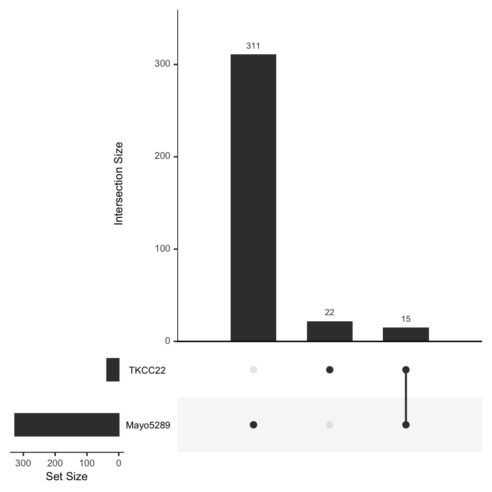
Figure 6.1: UpSet plot showing the relationship between the TKCC22 and Mayo-5289 experiments
Exercise 6.3
What are the genes in common? Hint: try the
interesectfunction!
6.8 Exporting results
Exporting results is straight forward! Results can also be stored in an .RData file for later use!
write.csv(as.data.frame(resMayo5289.Ordered), file = "resMayo5289.Ordered_results.csv")
save(dds, resMayo5289.Ordered, resTKCC22.Ordered, file = "PDCL_HNF4A_siRNA_Experiment.RData")
6.9 Data transformation and visualisation
For downstream analyses – e.g. for visualization or clustering – we need to work with transformed versions of the count data. There are a number of methods to transform count data provided in the DESeq2 package and include variance stabilizing transformations (vst) and regularized logarithm (rlog).
Both the vst and rlog transformations remove the dependence of the variance on the mean, particularly the high variance of the logarithm of count data when the mean is low. The vst and rlog transformations produce transformed data on the log2 scale which has been normalized with respect to library size and/or other normalization factors. The assay function returns the results of the transformation as a matrix of transformed values.
vsd <- vst(dds, blind=FALSE)
rld <- rlog(dds, blind=FALSE)
head(assay(vsd), 3)
#>                    HB.A1    HB.A3    HB.B1    HB.B3    HB.C1    HB.C3
#> ENSG00000227232 8.566844 8.611630 8.585389 8.633558 8.530630 8.541801
#> ENSG00000238009 7.239080 7.321780 7.438567 7.012016 7.263053 7.178992
#> ENSG00000237683 7.239080 7.351215 7.627718 7.414596 7.343795 7.402633
#>                    HB.D1    HB.D3    HB.E1    HB.E3    HB.F1    HB.F3
#> ENSG00000227232 8.688812 8.668386 8.761663 8.676995 8.490305 8.584954
#> ENSG00000238009 7.330801 7.288113 7.341380 7.289009 7.349144 7.252707
#> ENSG00000237683 7.833839 7.755957 7.742276 7.768123 7.794813 7.687399
6.9.1 PCA using transformed data
A well-established technique for visualization and extraction of relevant information is the popular Principal Component Analysis (PCA). PCA allows us to determine the relationship between samples and can provide valuable insights into the veracity of the results.
library(ggplot2)
pcaData <- plotPCA(vsd, intgroup=c("Treatment_group", "Batch"), returnData=TRUE)
percentVar <- round(100 * attr(pcaData, "percentVar"))
ggplot(pcaData, aes(PC1, PC2, color=Treatment_group, shape=as.factor(Batch))) +
  geom_point(size=3) +
  xlab(paste0("PC1: ",percentVar[1],"% variance")) +
  ylab(paste0("PC2: ",percentVar[2],"% variance"))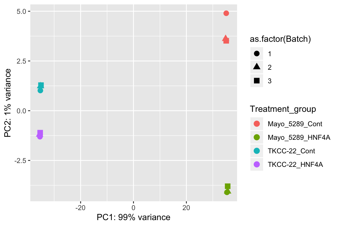
Figure 6.2: Principal Component Analysis (PCA) plot showing the relationship between the TKCC22 and Mayo-5289 experiments
6.9.2 Heatmaps using transformed data
Using vsd transformed data let’s generate a heatmap showing a selection of genes that are differentially expressed after HNF4A KD in the Mayo5289 cell line.
#Looking at the vsd matrix it comprises EnsemblIds and not gene symbols as row names!
head(assay(vsd), 3)
#>                    HB.A1    HB.A3    HB.B1    HB.B3    HB.C1    HB.C3
#> ENSG00000227232 8.566844 8.611630 8.585389 8.633558 8.530630 8.541801
#> ENSG00000238009 7.239080 7.321780 7.438567 7.012016 7.263053 7.178992
#> ENSG00000237683 7.239080 7.351215 7.627718 7.414596 7.343795 7.402633
#>                    HB.D1    HB.D3    HB.E1    HB.E3    HB.F1    HB.F3
#> ENSG00000227232 8.688812 8.668386 8.761663 8.676995 8.490305 8.584954
#> ENSG00000238009 7.330801 7.288113 7.341380 7.289009 7.349144 7.252707
#> ENSG00000237683 7.833839 7.755957 7.742276 7.768123 7.794813 7.687399
expMatrix <- assay(vsd)
#To make the Heatmap we will select genes based on our significant cutoffs
resMayo5289.Ordered <- resMayo5289.Ordered[!is.na(resMayo5289.Ordered$symbol),]

resMayo5289.select <- subset(resMayo5289.Ordered,
                             padj <= 1e-20 &
                               abs(resMayo5289.Ordered$log2FoldChange) >= 1)
#Map the significant results to the transformed expression values
inter <- intersect(rownames(expMatrix), rownames(resMayo5289.select))
head(inter)
#> [1] "ENSG00000162545" "ENSG00000137959" "ENSG00000198758" "ENSG00000134193"
#> [5] "ENSG00000198483" "ENSG00000163209"
#Subset the matrix to include only the significant genes of interest
expMatrix.select <- expMatrix[inter, ]
dim(expMatrix.select)
#> [1] 82 12
head(expMatrix.select)
#>                     HB.A1     HB.A3     HB.B1     HB.B3     HB.C1     HB.C3
#> ENSG00000162545 10.895563 10.600985 10.910440 10.657951 10.842195 10.633991
#> ENSG00000137959  7.387884  7.580602  7.246242  7.513228  7.292596  7.467657
#> ENSG00000198758 10.109697  9.496844 10.195344  9.511486 10.207478  9.498285
#> ENSG00000134193  7.906800  7.876837  7.934171  7.830890  7.870031  7.882784
#> ENSG00000198483  7.172658  7.289183  7.203331  7.280885  7.012016  7.216462
#> ENSG00000163209  7.332804  7.378253  7.416824  7.280885  7.292596  7.130119
#>                     HB.D1     HB.D3     HB.E1     HB.E3    HB.F1     HB.F3
#> ENSG00000162545 11.092906 10.173745 11.041170 10.154572 11.05369 10.048354
#> ENSG00000137959 10.489250 11.855465 10.855140 12.085880 10.74541 11.910030
#> ENSG00000198758 11.218128 10.317309 11.248313 10.373998 11.20353 10.299625
#> ENSG00000134193 11.622704 10.881198 11.747548 10.706791 11.75830 10.660777
#> ENSG00000198483  8.229145  9.195484  8.268459  9.225827  8.18042  9.111117
#> ENSG00000163209 10.769595  9.569257 10.669877  9.599853 10.55096  9.571898
Let’s now finish off the matrix by swapping the Ensembl IDs for the gene symbols - this will make our heatmap biologist friendly! We also want to limit the matrix to the Mayo5289 HNF4A KD experiment!
#Add human readable gene names
rownames(expMatrix.select) <- mapIds(org.Hs.eg.db,
                     keys=rownames(expMatrix.select),
                     column="SYMBOL",
                     keytype="ENSEMBL",
                     multiVals="first")
#> 'select()' returned 1:1 mapping between keys and columns
head(rownames(expMatrix.select))
#> ENSG00000162545 ENSG00000137959 ENSG00000198758 ENSG00000134193
#>       "CAMK2N1"        "IFI44L"        "EPS8L3"          "REG4"
#> ENSG00000198483 ENSG00000163209
#>       "ANKRD35"         "SPRR3"
#Select the Mayo5289 columns
expMatrix.select <- expMatrix.select[, grepl("Mayo_5289_HNF4A|Mayo_5289_Cont",colData(dds)$Treatment_group)]
#Give the matrix some useful column names
colnames(expMatrix.select) <- colData(dds)[colnames(expMatrix.select),"Treatment_group"]
head(expMatrix.select)
#>         Mayo_5289_Cont Mayo_5289_HNF4A Mayo_5289_Cont Mayo_5289_HNF4A
#> CAMK2N1      11.092906       10.173745      11.041170       10.154572
#> IFI44L       10.489250       11.855465      10.855140       12.085880
#> EPS8L3       11.218128       10.317309      11.248313       10.373998
#> REG4         11.622704       10.881198      11.747548       10.706791
#> ANKRD35       8.229145        9.195484       8.268459        9.225827
#> SPRR3        10.769595        9.569257      10.669877        9.599853
#>         Mayo_5289_Cont Mayo_5289_HNF4A
#> CAMK2N1       11.05369       10.048354
#> IFI44L        10.74541       11.910030
#> EPS8L3        11.20353       10.299625
#> REG4          11.75830       10.660777
#> ANKRD35        8.18042        9.111117
#> SPRR3         10.55096        9.571898
We now make the heatmap using the ComplexHeatmap package.
library(ComplexHeatmap)
library(circlize)
#Define some colours for the annotation
colors <- RColorBrewer::brewer.pal(8, "Set1")
#Make the sample annotation track
ha <- HeatmapAnnotation(Treatment = colnames(expMatrix.select),
                        col = list(Treatment = structure(names = c(
                          "Mayo_5289_Cont", "Mayo_5289_HNF4A"
                        ), colors[3:4])))
#Scale the matrix to generate z-scores
expMatrix.select.sc <- t(scale(t(expMatrix.select)))
#Generate the heatmap
Heatmap(
  expMatrix.select.sc,
  col = colorRamp2(c(-2, 0, 2), c("#377EB8", "white", "#E41A1C")),
  name = "Z score",
  cluster_columns = TRUE,
  cluster_rows = TRUE,
  top_annotation = ha,
  show_row_names = TRUE,
  show_column_names = FALSE, #Turned off column names
  row_names_gp = gpar(fontsize = 5),
  column_names_gp = gpar(fontsize = 5)
)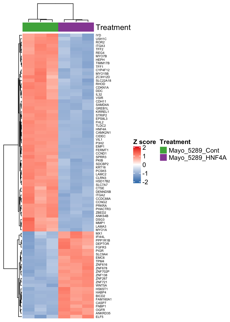
Figure 6.3: Heatmap showing differentially expressed genes in Mayo-5289 after HNF4A KD
6.10 Gene Set Enrichment Analysis
Over-representation and/or Gene Set Enrichment Analysis (GSEA) are essential tasks in any RNAseq study. These analyses help to define biological functions and/or processes that are enriched in different biological samples. In this section we will use the clusterProfiler package to perform over-representation analysis to determine whether known biological functions or processes are over-represented (= enriched) in an experimentally-derived gene list, e.g. a list of differentially expressed genes (DEGs). A comprehensive overview of the theory and methods used in this section is provided at the following location clusterProfiler-book or by typing browseVignettes("clusterProfiler") at the R prompt. Please read through the clusterProfiler documentation.
First load the clusterProfiler library into the current environment.
library(clusterProfiler)For over-representation analysis, we require a vector of gene IDs. These gene IDs can be obtained by differential expression analysis (e.g. with the DESeq2 package). The functions that we will be using require Entrez IDs as input. We define a vector of significantly and differentially expressed Entrez IDs (genes) defining our experiment as follows:
resMayo5289.enriched <- subset(resMayo5289.Ordered,
                               padj <= 0.05)
6.10.1 KEGG
KEGG (Kyoto Encyclopedia of Genes and Genomes) is a collection of databases dealing with genomes, biological pathways, diseases, drugs, and chemical substances. Our analysis will determine whether our experimentally derived gene list is enriched in any one of the curated gene sets defined by KEGG. To do this we will use the enrichKEGG function.
#Perform the over-representation analysis using keggEnrich
keggEnrich <- enrichKEGG(gene = resMayo5289.enriched$entrez,
                         organism     = 'hsa',
                         pvalueCutoff = 0.05)
head(keggEnrich)
#>                ID                            Description GeneRatio  BgRatio
#> hsa04390 hsa04390                Hippo signaling pathway   52/1613 157/8094
#> hsa05418 hsa05418 Fluid shear stress and atherosclerosis   47/1613 139/8094
#> hsa05222 hsa05222                 Small cell lung cancer   34/1613  92/8094
#> hsa04068 hsa04068                 FoxO signaling pathway   44/1613 131/8094
#> hsa04115 hsa04115                  p53 signaling pathway   28/1613  73/8094
#> hsa00600 hsa00600                Sphingolipid metabolism   21/1613  49/8094
#>                pvalue   p.adjust      qvalue
#> hsa04390 5.990875e-05 0.01125709 0.008723608
#> hsa05418 7.560810e-05 0.01125709 0.008723608
#> hsa05222 1.043490e-04 0.01125709 0.008723608
#> hsa04068 1.507906e-04 0.01125709 0.008723608
#> hsa04115 2.012321e-04 0.01125709 0.008723608
#> hsa00600 2.071857e-04 0.01125709 0.008723608
#>                                                                                                                                                                                                                                                                         geneID
#> hsa04390 595/166824/7474/84962/122786/330/652/7042/6657/6591/80326/71/3398/84612/1495/27113/1741/7532/25937/4092/4088/999/1490/5516/10413/1499/7476/7533/332/81029/5522/9231/8312/374/60/7534/23513/7004/329/1856/3996/2736/51176/7046/8324/60485/1454/5520/650/2535/7855/7473
#> hsa05418                                      7850/4259/652/5154/858/71/2948/207/3162/7295/445/91860/801/8878/6300/3685/5747/3320/5879/1499/5599/7157/2938/9446/5602/60/6382/5562/5155/4780/1843/90/5563/10365/6613/1728/3326/2946/8503/6416/1535/9181/7422/805/3725/5600/4217
#> hsa05222                                                                                                  595/3918/3909/1026/3673/3675/330/4616/1647/1284/207/3914/7187/6257/3685/598/1021/51426/3688/5747/54205/3913/836/7185/7157/1869/3655/329/1287/331/5728/8503/6502/1027
#> hsa04068                                         595/1026/80854/901/7042/4616/9455/5106/1647/207/5565/604/6789/6300/4088/1263/6774/5599/10769/3276/6446/8743/4193/3643/3667/10110/5602/1956/5562/664/7046/5563/10365/6794/92579/1454/5728/8503/85417/51422/2308/6502/1027/5600
#> hsa04115                                                                                                                        595/1026/901/2810/64065/3732/4616/8795/5268/1647/27113/9540/598/1021/637/54205/64393/836/7157/8797/4193/50484/84883/3486/55240/5728/7249/51246
#> hsa00600                                                                                                                                                     2581/29956/8612/123099/57704/8877/9517/64781/81537/55627/2717/410/6609/8611/9514/8879/8560/2629/79603/55331/56848
#>          Count
#> hsa04390    52
#> hsa05418    47
#> hsa05222    34
#> hsa04068    44
#> hsa04115    28
#> hsa00600    21
#Make the output biologist friendly
keggEnrichRead <-
  setReadable(keggEnrich, OrgDb = org.Hs.eg.db, keyType = "ENTREZID")
head(keggEnrichRead, 55)
#>                ID                            Description GeneRatio  BgRatio
#> hsa04390 hsa04390                Hippo signaling pathway   52/1613 157/8094
#> hsa05418 hsa05418 Fluid shear stress and atherosclerosis   47/1613 139/8094
#> hsa05222 hsa05222                 Small cell lung cancer   34/1613  92/8094
#> hsa04710 hsa04710                       Circadian rhythm   13/1613  31/8094
#> hsa05225 hsa05225               Hepatocellular carcinoma   48/1613 168/8094
#> hsa01230 hsa01230            Biosynthesis of amino acids   25/1613  75/8094
#>                pvalue   p.adjust      qvalue
#> hsa04390 5.990875e-05 0.01125709 0.008723608
#> hsa05418 7.560810e-05 0.01125709 0.008723608
#> hsa05222 1.043490e-04 0.01125709 0.008723608
#> hsa04710 4.176224e-03 0.04644364 0.035991197
#> hsa05225 4.194968e-03 0.04644364 0.035991197
#> hsa01230 4.273955e-03 0.04644364 0.035991197
#>                                                                                                                                                                                                                                                                                                                  geneID
#> hsa04390 CCND1/RASSF6/WNT5A/AJUBA/FRMD6/BIRC3/BMP4/TGFB2/SOX2/SNAI2/WNT10A/ACTG1/ID2/PARD6B/CTNNA1/BBC3/DLG3/YWHAG/WWTR1/SMAD7/SMAD3/CDH1/CCN2/PPP2CB/YAP1/CTNNB1/WNT7A/YWHAH/BIRC5/WNT5B/PPP2R2C/DLG5/AXIN1/AREG/ACTB/YWHAZ/SCRIB/TEAD4/BIRC2/DVL2/LLGL1/GLI2/LEF1/TGFBR1/FZD7/SAV1/CSNK1E/PPP2R2A/BMP2/FZD2/FZD5/WNT3
#> hsa05418                  IL1R2/MGST3/BMP4/PDGFA/CAV2/ACTG1/GSTM4/AKT1/HMOX1/TXN/ASS1/CALML4/CALM1/SQSTM1/MAPK12/ITGAV/PTK2/HSP90AA1/RAC1/CTNNB1/MAPK8/TP53/GSTA1/GSTO1/MAPK10/ACTB/SDC1/PRKAA1/PDGFB/NFE2L2/DUSP1/ACVR1/PRKAA2/KLF2/SUMO2/NQO1/HSP90AB1/GSTM2/PIK3R3/MAP2K4/CYBA/ARHGEF2/VEGFA/CALM2/JUN/MAPK11/MAP3K5
#> hsa05222                                                                                                     CCND1/LAMC2/LAMA3/CDKN1A/ITGA2/ITGA3/BIRC3/GADD45B/GADD45A/COL4A2/AKT1/LAMB3/TRAF3/RXRB/ITGAV/BCL2L1/CDK6/POLK/ITGB1/PTK2/CYCS/LAMB2/CASP3/TRAF1/TP53/E2F1/ITGA6/BIRC2/COL4A5/XIAP/PTEN/PIK3R3/SKP2/CDKN1B
#> hsa04710                                                                                                                                                                                                                                BHLHE41/PRKAB2/PER3/CREB1/PER2/PER1/NR1D1/PRKAA1/CRY1/PRKAA2/RORC/CSNK1E/PRKAG2
#> hsa05225                CCND1/CDKN1A/MGST3/WNT5A/FRAT2/TGFB2/GADD45B/WNT10A/TGFA/ACTG1/GADD45A/GSTM4/AKT1/HMOX1/MET/TXNRD1/BCL2L1/CDK6/POLK/SMAD3/SMARCE1/CTNNB1/WNT7A/WNT5B/TP53/AXIN1/E2F1/SMARCC1/GSTA1/GSTO1/BRD7/ACTB/EGFR/GAB1/DVL2/NFE2L2/LEF1/TGFBR1/NQO1/FZD7/PTEN/GSTM2/PIK3R3/FZD2/SMARCD2/FZD5/SMARCD3/WNT3
#> hsa01230                                                                                                                                                                                  PSAT1/GLUL/PFKL/GPT2/ACO2/ACO1/CBS/ASS1/SHMT1/PHGDH/RPIA/ASNS/ALDOB/TKT/IDH3A/IDH1/IDH2/PSPH/IDH3G/CS/ENO2/ENO1/PFKP/PC/PYCR3
#>          Count
#> hsa04390    52
#> hsa05418    47
#> hsa05222    34
#>  ...<24 more rows>...
#> hsa04710    13
#> hsa05225    48
#> hsa01230    25
6.10.2 REACTOME
Like KEGG, the REACTOME database contains curated gene set annotations covering diverse molecular and cellular biology pathways. Similarly, our analysis will determine whether our experimentally derived gene list is enriched in any one of the curated gene sets defined by REACTOME. To do this we use the enrichPathway function provided by the ReactomePA package.
library(ReactomePA)
reactomeEnrich <- enrichPathway(
  gene = resMayo5289.enriched$entrez,
  organism = "human",
  pvalueCutoff = 0.05,
  pAdjustMethod = "BH",
  qvalueCutoff = 0.2,
  minGSSize = 10,
  maxGSSize = 500,
  readable = TRUE
)
head(reactomeEnrich, 5)
#>                          ID                                      Description
#> R-HSA-1059683 R-HSA-1059683                          Interleukin-6 signaling
#> R-HSA-112409   R-HSA-112409               RAF-independent MAPK1/3 activation
#> R-HSA-5357801 R-HSA-5357801                            Programmed Cell Death
#> R-HSA-109581   R-HSA-109581                                        Apoptosis
#> R-HSA-5633008 R-HSA-5633008 TP53 Regulates Transcription of Cell Death Genes
#>               GeneRatio   BgRatio       pvalue   p.adjust     qvalue
#> R-HSA-1059683    9/2199  11/10619 2.521779e-05 0.01521919 0.01419629
#> R-HSA-112409    14/2199  23/10619 3.112841e-05 0.01521919 0.01419629
#> R-HSA-5357801   60/2199 179/10619 3.891784e-05 0.01521919 0.01419629
#> R-HSA-109581    59/2199 176/10619 4.485219e-05 0.01521919 0.01419629
#> R-HSA-5633008   21/2199  44/10619 5.518197e-05 0.01521919 0.01419629
#>                                                                                                                                                                                                                                                                                                                                                                         geneID
#> R-HSA-1059683                                                                                                                                                                                                                                                                                                               SOCS3/IL6ST/STAT1/TYK2/IL6R/STAT3/JAK2/PTPN11/JAK1
#> R-HSA-112409                                                                                                                                                                                                                                                                                 IL6ST/DUSP4/TYK2/IL6R/JAK2/DUSP6/PTPN11/DUSP10/DUSP7/DUSP1/JAK1/PEA15/DUSP2/DUSP5
#> R-HSA-5357801 CASP7/SFN/DSG3/BIRC3/TJP2/TNFRSF10B/PLEC/PSMB8/UACA/AKT1/MAGED1/NMT1/BBC3/BCL2L1/YWHAG/BID/CDH1/PTK2/TLR4/PSMC3/CTNNB1/RIPK1/CYCS/STAT3/MAPK8/PSME2/YWHAH/GSN/CASP3/DSP/PSMC4/H1F0/TP53/UNC5A/TNFRSF10A/TNFSF10/PSME1/E2F1/APIP/PPP3CC/PSMB9/YWHAZ/BMF/BIRC2/SPTAN1/ARHGAP10/APPL1/XIAP/UBB/HIST1H1C/DBNL/TJP1/FADD/PSMD7/TICAM1/PRKCQ/TP63/HIST1H1E/LMNB1/PSMD1
#> R-HSA-109581        CASP7/SFN/DSG3/TJP2/TNFRSF10B/PLEC/PSMB8/UACA/AKT1/MAGED1/NMT1/BBC3/BCL2L1/YWHAG/BID/CDH1/PTK2/TLR4/PSMC3/CTNNB1/RIPK1/CYCS/STAT3/MAPK8/PSME2/YWHAH/GSN/CASP3/DSP/PSMC4/H1F0/TP53/UNC5A/TNFRSF10A/TNFSF10/PSME1/E2F1/APIP/PPP3CC/PSMB9/YWHAZ/BMF/BIRC2/SPTAN1/ARHGAP10/APPL1/XIAP/UBB/HIST1H1C/DBNL/TJP1/FADD/PSMD7/TICAM1/PRKCQ/TP63/HIST1H1E/LMNB1/PSMD1
#> R-HSA-5633008                                                                                                                                                                                                                   PERP/TNFRSF10B/TP53INP1/BCL6/BBC3/TP53I3/BID/PRELID1/CASP10/CASP1/BIRC5/TP53/BNIP3L/TNFRSF10A/NDRG1/AIFM2/IGFBP3/STEAP3/RABGGTB/TP63/TNFRSF10D
#>               Count
#> R-HSA-1059683     9
#> R-HSA-112409     14
#> R-HSA-5357801    60
#> R-HSA-109581     59
#> R-HSA-5633008    21
6.10.3 Plotting functions
Once we have our results, we would like to generate publication quality figures. The clusterProfiler and enrichPlot packages provide a number of plotting functions that make this easy.
Dotplot
library(enrichplot)
plot1 <- dotplot(keggEnrich, showCategory = 10) + ggtitle("KEGG")
#> wrong orderBy parameter; set to default `orderBy = "x"`
plot2 <-
  dotplot(reactomeEnrich, showCategory = 10) + ggtitle("REACTOME")
#> wrong orderBy parameter; set to default `orderBy = "x"`
plot_grid(plot1, plot2, ncol = 2)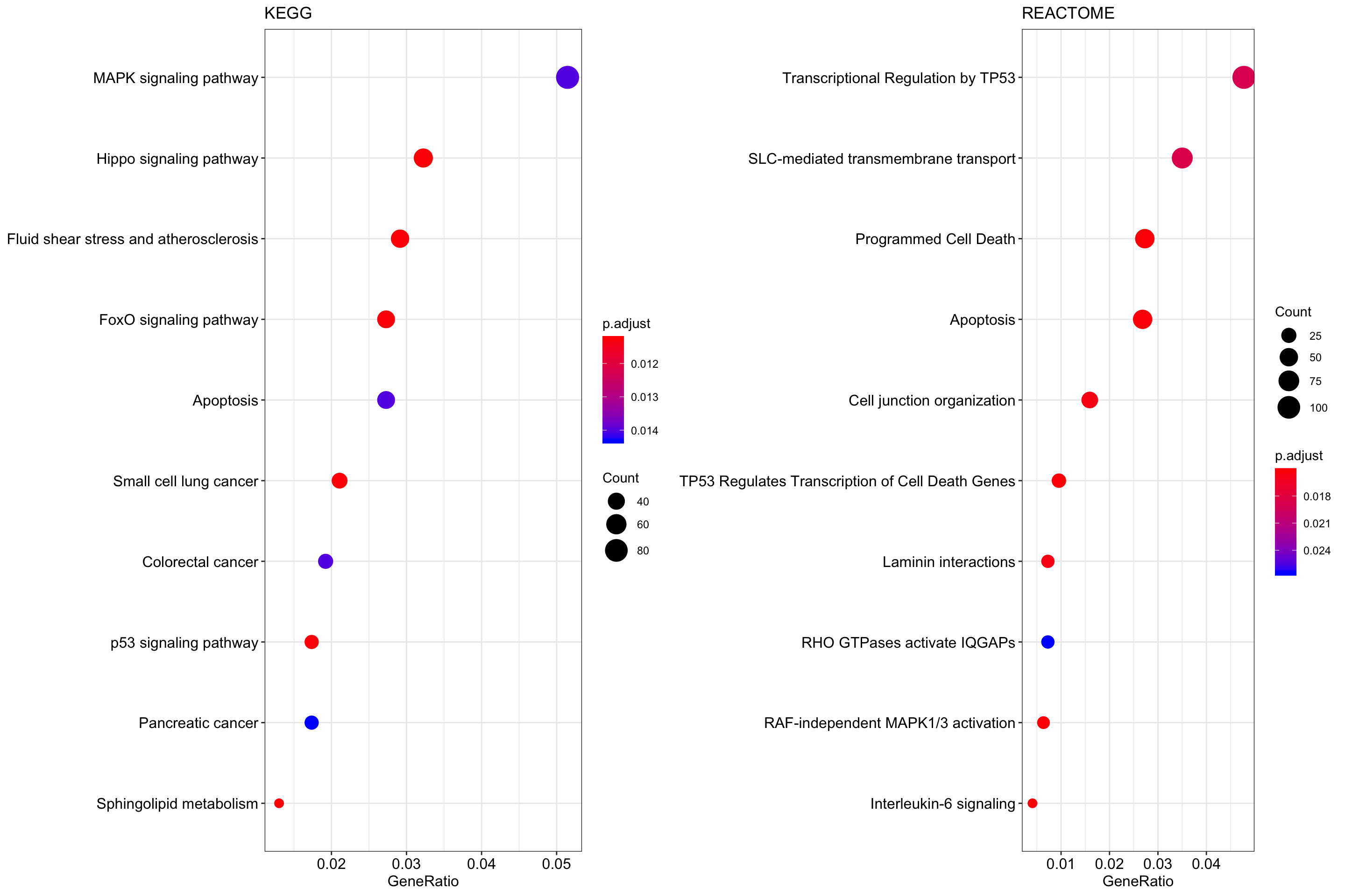
Figure 6.4: Dotplot showing KEGG and REACTOME pathways that are significantly enriched.
Upset plot
An upsetplot shows the overlap of genes comprising different gene sets and provides a complex overview of genes and gene sets significantly enriched in the experiment.
upsetplot(reactomeEnrich) 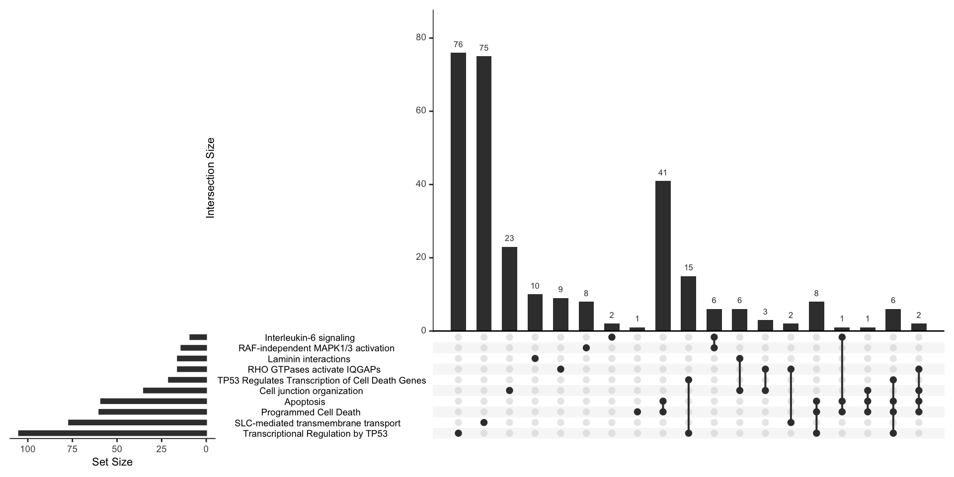
Figure 6.5: UpSet plot showing the overlap of genes comprising significantly enriched processes and pathways.
Enrichment map plot
An enrichment map plot emapplot generates a network of significantly enriched gene sets with edges connecting overlapping gene sets.
emapplot(reactomeEnrich)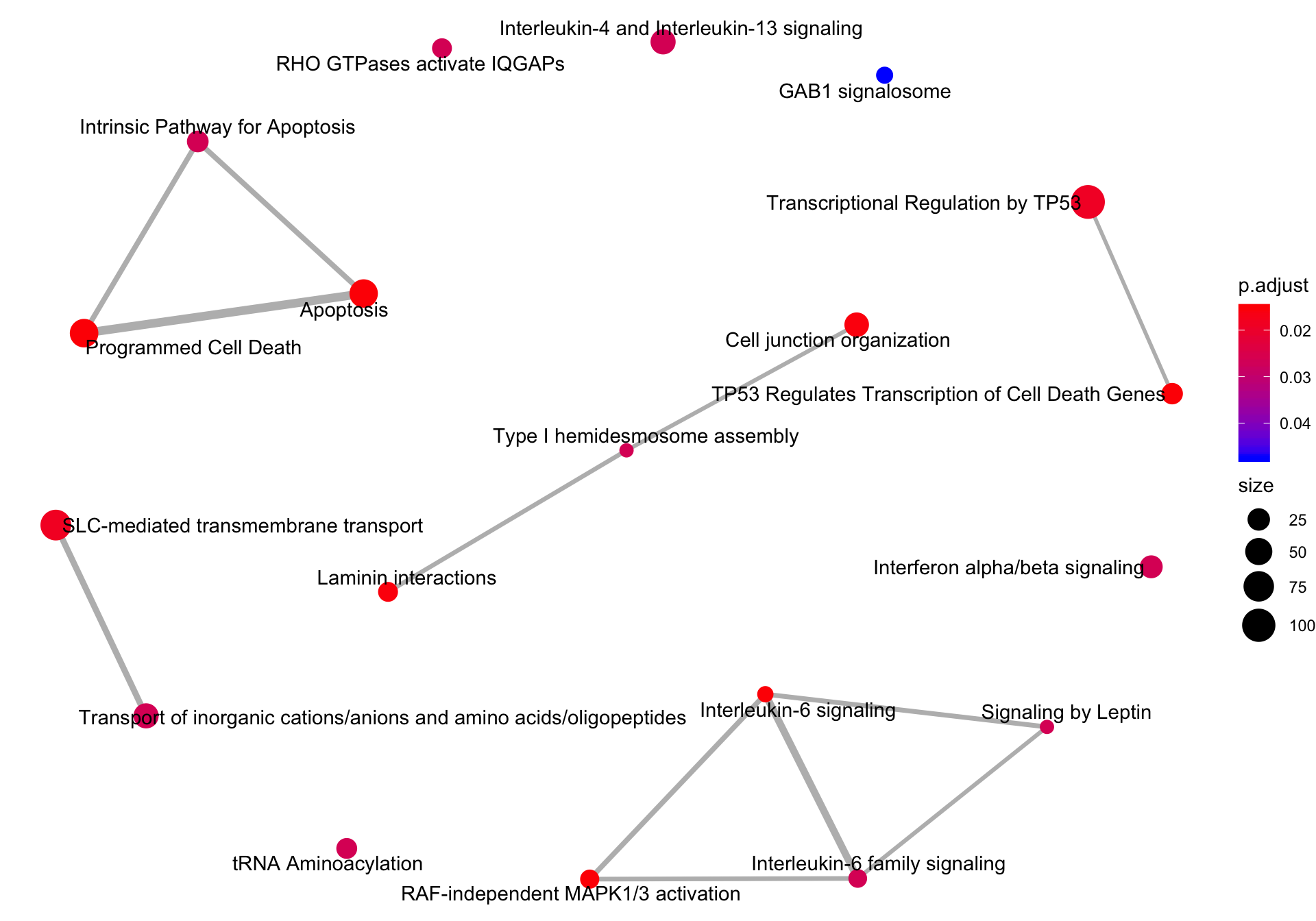
Figure 6.6: Enrichment map of Reactome pathways significantly enriched.
6.10.4 Extracting enrichment results to generate heatmaps
The above analysis showed that our experimentally derived gene list is significantly enriched in the “Transcriptional Regulation by TP53” REACTOME gene set. Because we have selected genes that are both up and down regulated following HNF4A KD, we would like to understand how specific genes, within this pathway, are modulated by HNF4A. A heatmap is an informative way of determining the relative expression of sets of genes, so let’s generate a heatmap using the set of genes comprising this pathway. First, we need to get the data into the correct shape as follows:
slotNames(reactomeEnrich)
#>  [1] "result"        "pvalueCutoff"  "pAdjustMethod" "qvalueCutoff"
#>  [5] "organism"      "ontology"      "gene"          "keytype"
#>  [9] "universe"      "gene2Symbol"   "geneSets"      "readable"
reactResults <- reactomeEnrich@result
tp53genes <- subset(reactResults,
                    Description == "Transcriptional Regulation by TP53")$geneID
tp53genes.vector <- strsplit(tp53genes, "/")[[1]]
expMatrix <- assay(vsd)
rownames(expMatrix) <- mapIds(
  org.Hs.eg.db,
  keys = rownames(expMatrix),
  column = "SYMBOL",
  keytype = "ENSEMBL",
  multiVals = "first"
)
#> 'select()' returned 1:many mapping between keys and columns
#Map the significant results to the transformed expression values
inter <- intersect(rownames(expMatrix), tp53genes.vector)
expMatrix.tp53 <- expMatrix[inter,]
#Add human readable gene names
expMatrix.tp53 <- expMatrix.tp53[, grepl("Mayo_5289_HNF4A|Mayo_5289_Cont",
                         colData(dds)$Treatment_group)]
#Give the matrix some useful column names
colnames(expMatrix.tp53) <-
  colData(dds)[colnames(expMatrix.tp53), "Treatment_group"]
Notice that we have used the
strsplitfunction to split the character stringtp53genesinto a vector of gene symbols!
Now produce the heatmap using the ComplexHeatmap package:
#Setup the annotation showing treatment type
ha <- HeatmapAnnotation(Treatment = colnames(expMatrix.tp53),
                        col = list(Treatment = structure(
                          names = c("Mayo_5289_Cont", "Mayo_5289_HNF4A"), colors[3:4]
                        )))
#Scale the matrix to generate z-scores
expMatrix.tp53.sc <- t(scale(t(expMatrix.tp53)))
#Generate the heatmap
Heatmap(
  expMatrix.tp53.sc,
  col = colorRamp2(c(-2, 0, 2), c("#377EB8", "white", "#E41A1C")),
  name = "Z score",
  cluster_columns = TRUE,
  cluster_rows = TRUE,
  top_annotation = ha,
  show_row_names = TRUE,
  show_column_names = FALSE,
  #Turned off column names
  row_names_gp = gpar(fontsize = 5),
  column_names_gp = gpar(fontsize = 5)
)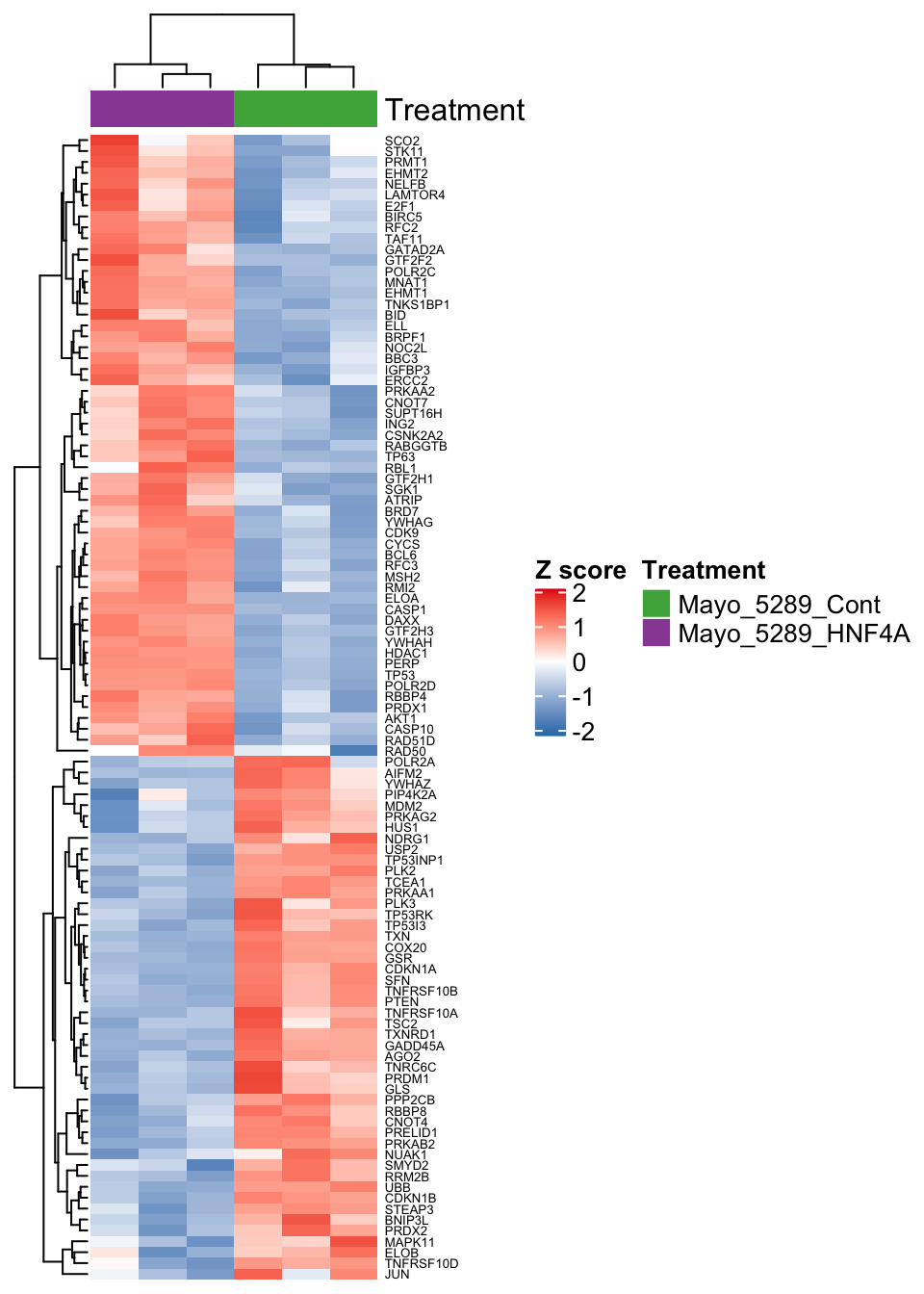
Figure 6.7: Heatmap showing differentially expressed genes in the Transcriptional Regulation by TP53 Reactome pathway